Machine Learning for Diabetes Risk Prediction

The CDC BRFSS 2015 survey records 253,680 respondents with 21 features covering health status, lifestyle, and demographics. The target variable Diabetes_012 is three-category (0: no diabetes, 1: prediabetes, 2: diabetes), transformed into a binary at-risk label (At-risk = Diabetes_012 ≥ 1) for classification. The diabetes outcome is notably imbalanced — most individuals are classified as no-diabetes — motivating class weighting and threshold-based evaluation.

This project addresses two objectives: individual-level risk prediction through classification, and population-level segmentation through clustering. The workflow follows CRISP-DM.

Figure 1. Class distribution of the diabetes outcome; the at-risk class (prediabetes + diabetes) accounts for roughly 14% of respondents

Dataset and preparation

No missing values. 9.42% of records share identical responses — retained to preserve population distribution, as no unique respondent identifier exists. All features are already numerically encoded (binary or ordinal). Standardisation applied selectively: only for logistic regression; tree-based models trained on unscaled features.

For clustering, only the 14 health status and lifestyle features were retained — they more directly reflect population health profiles than demographics. Correlation and variance-based checks found no highly correlated or near-zero variance features among these 14.

Classification models

Feature selection via RFECV (LR estimator, stratified CV, ROC-AUC scoring) found that cross-validated AUC plateaued at 0.818 with all 21 features retained — no benefit from removal. All features were kept for modelling.

Figure 2. RFECV performance curve — cross-validated ROC-AUC plateaus at 0.818 across all 21 features, confirming no gain from feature removal

Experiments included: (1) baseline vs tuned LR (GridSearchCV over C), (2) baseline vs tuned RF (RandomizedSearchCV), (3) tuned model comparison at t = 0.5, (4) class-weighted vs SMOTE, and (5) cost-sensitive threshold optimisation for healthcare deployment.

Figure 3. LR baseline vs tuned — ROC and PR curves are near-identical; tuning yields no meaningful gain (AUC 0.818 for both)

Figure 4. RF baseline vs tuned — marginal improvement from tuning (AUC 0.818 → 0.821); no meaningful change in minority class performance

Model	ROC-AUC	AP	At-risk Recall	F1
LR baseline	0.818	0.433	—	—
LR tuned (C=0.05)	0.818	0.433	0.761	0.470
RF baseline	0.818	0.453	—	—
RF tuned	0.821	0.456	0.746	0.456
LR + SMOTE	0.815	—	0.753	0.468

CV ROC-AUC for final LR: 0.8177 (test: 0.8176) — stable generalisation. Tuning yields no meaningful improvement for either model.

LR vs RF

Figure 5. Confusion matrices at t = 0.5 — LR achieves higher at-risk recall (0.761 vs 0.746), meaning fewer missed at-risk cases under the same threshold

Under t = 0.5, LR achieves higher at-risk recall (0.761 vs 0.746) — fewer false negatives, more critical for the screening objective. The real distinction comes from the cost curve. LR reaches minimum expected cost at t = 0.48 with a flat, smooth curve — robust to threshold variation. RF requires t = 0.16 and its cost curve is steep, highly sensitive to small threshold changes.

Figure 10. Cost-sensitive threshold analysis — LR minimises cost at t = 0.48 with a flat curve; RF requires t = 0.16 and is fragile to small threshold shifts

LR selected as the final model. Not for AUC, but for stable and interpretable operating behaviour suited to screening where missed at-risk cases are costly.

Class weighting vs SMOTE

Figure 6. SMOTE vs class-weighted LR — both approaches produce nearly identical ROC-AUC, recall, and F1; class weighting retained for lower complexity

SMOTE-based LR closely matches class-weighted LR (ROC-AUC 0.815 vs 0.818, recall 0.753 vs 0.761, F1 0.468 vs 0.470). No meaningful gain — class weighting retained given lower complexity.

Threshold sensitivity

Figure 9. Threshold sensitivity — as t increases, recall falls sharply while precision rises; LR consistently maintains slightly higher recall than RF across most thresholds

Comparison and calibration

Figure 7. Full model comparison — LR and RF achieve near-identical ROC-AUC and PR curves; neither is well-calibrated across the full probability range

Neither model is well-calibrated across the full probability range. LR exhibits conservative estimates at higher predicted risk levels. Uncalibrated RF shows substantial miscalibration; after isotonic regression, RF probabilities align more closely with the ideal calibration diagonal. Explicit calibration is required before outputs are used for individual-level risk communication.

Figure 8. Calibration curves — LR is conservative at high risk levels; RF improves substantially after isotonic regression calibration

Final model: LR tuned at t = 0.48. ROC-AUC 0.8176, at-risk recall 0.7606, accuracy 0.7303, 1,914 false negatives.

SHAP interpretability

SHAP confirms predictions are driven by a small set of health-related factors with clear directional effects.

Feature	Mean SHAP	Direction
GenHlth	0.50	Poorer self-reported health → ↑ risk
Age	0.38	Older age → ↑ risk
BMI	0.35	Higher BMI → ↑ risk
HighBP	0.34	Hypertension present → ↑ risk
HighChol	0.29	High cholesterol → ↑ risk

Figure B3. SHAP explanations for the final logistic regression model — global importance (bar), value distribution (beeswarm), and individual explanation (waterfall); GenHlth, Age, BMI, HighBP, and HighChol dominate with clear directional effects

At the individual level, high-risk classifications arise from the cumulative contribution of dominant factors rather than any single extreme value. Protective attributes — absence of chronic conditions — partially offset risk but rarely dominate.

Clustering models

k selection

k=2 achieves a high silhouette score but represents only a coarse binary separation. k=6 yields slightly higher scores under PCA(6) but is inconsistent under PCA(10) — suggesting over-segmentation. k=3 is stable across both representations and was selected, balancing quality, robustness, and interpretability.

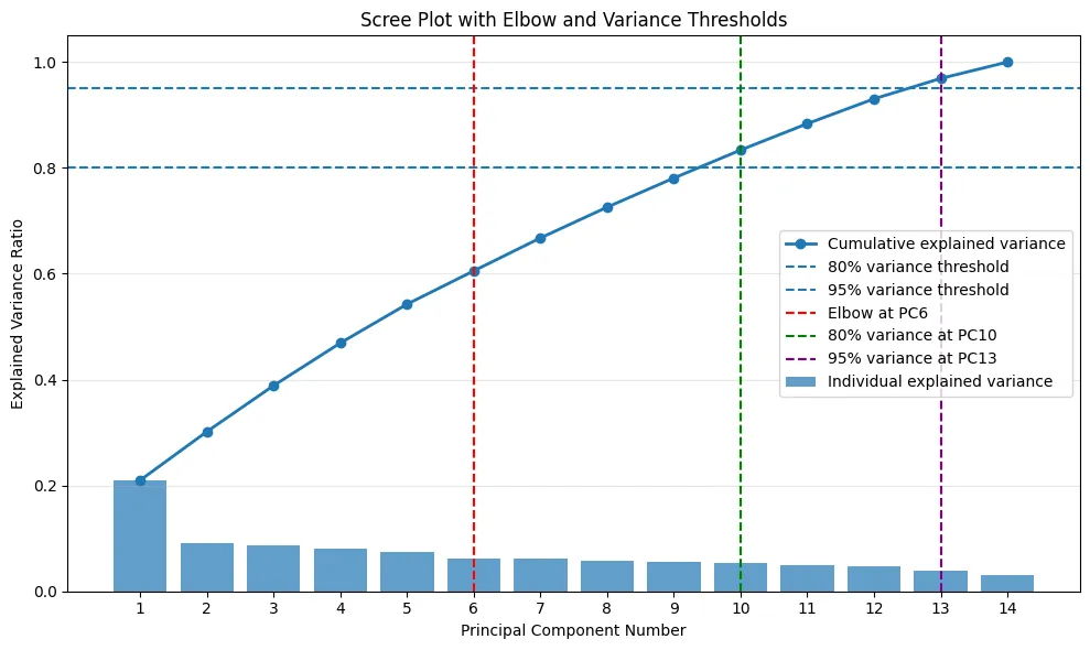
Figure 11. Scree plot — cumulative variance reaches 60.55% at PC6 (elbow), justifying PCA(6) as the primary representation; PCA(10) retained at 83.38% for robustness comparison

Figure 12. K-means silhouette scores for k = 2–8 under PCA(6) and PCA(10) — k=3 is stable across both representations; k=6 is sensitive to dimensionality choice

PCA(6) vs PCA(10), K-means vs Hierarchical

Method	Silhouette	WCSS	Note
K-means PCA(6) k=3	0.197	1,440,681	Smooth, balanced — selected
K-means PCA(10) k=3	similar	higher	Cluster 2 compressed, less balanced
Hierarchical PCA(6) k=3	0.297	higher	One dominant cluster, size imbalance

PCA(6) shows smoother transitions between clusters along PC1, which better reflects gradual health variation. Hierarchical clustering achieves a higher silhouette score but concentrates most samples into a single dominant cluster — K-means produces more evenly sized, interpretable partitions.

Figure 13. K-means (k=3) under PCA(6) and PCA(10) in PC1–PC2 space — separation is primarily driven by PC1; PCA(10) sharpens boundaries but compresses Cluster 2

Figure 14. Hierarchical dendrogram (PCA-6, Ward linkage, subsample) — clear two-branch split at top level, supporting k=3

Figure 15. Silhouette comparison — hierarchical clustering achieves higher mean score (0.297 vs 0.197) but concentrates samples in a single cluster; K-means produces a more balanced partition

Cluster health profiles

The three clusters exhibit clearly differentiated health patterns and distinct diabetes risk compositions (chi-square confirms external validity).

	Cluster 0	Cluster 1	Cluster 2
Label	Low Risk	Lifestyle-driven	High Clinical Burden
BMI	Low	Moderate	High
GenHlth / PhysHlth	Good	Moderate	Poor
HighBP / HighChol / CVD	Low	Low–moderate	High
Physical activity	Moderate	Low	Low
Smoking / Alcohol	Low	High	Moderate
Diabetes composition	Lowest	Moderate	Highest
Intervention	Preventive	Lifestyle change	Clinical management

Figure 16. Cluster profiles — standardised means heatmap; Cluster 2 shows consistently elevated risk indicators across all dimensions

Figure 17. Diabetes distribution across clusters — chi-square confirms external validity; Cluster 2 has the highest diabetes prevalence

Cluster 0 shows generally favourable health indicators — lower BMI, fewer chronic conditions, and better self-reported health — representing a low-risk profile suited to preventive health maintenance. Cluster 1 is characterised primarily by lifestyle-related differences, particularly in physical activity, smoking, and dietary behaviours, despite relatively moderate clinical risk, indicating a need for behaviour-focused lifestyle interventions. Cluster 2 displays consistently elevated levels across multiple adverse health indicators, including BMI, poor general health, cardiovascular conditions, and mobility limitations — a high-risk profile driven by accumulated clinical burden that warrants targeted clinical management and monitoring.

The clear separation of health profiles across all three clusters supports the external validity of the clustering solution and its potential application in population-level diabetes risk stratification.

Reflection

Why LR over RF? Not AUC — both are comparable. The decision rests on the cost curve shape. LR’s flat minimum around t ≈ 0.48 means deployment threshold can be varied without sharply increasing cost. RF’s steep minimum at t ≈ 0.16 is fragile.

Why k=3? Not the highest silhouette — but the most stable across PCA representations. As Hennig (2007) notes: a meaningful cluster should not disappear easily when the data is changed in a non-essential way.

Limitations: BRFSS is cross-sectional — causality cannot be inferred. Both models lack reliable probability calibration across the full risk range. Clustering is sensitive to feature selection scope and PCA dimensionality choice.